RNN-T in Automatic Speech Recognition
The article explores the architecture and training processes of the RNN-T model in ASR.
Introduction
In this blog post, we will briefly discuss the popular transducer based model- RNN-T in speech recognition. It does not discuss everything from one particular paper but represents my understanding from multiple sources and Lugosch, 2020’s blog on the same topic. Lately, these models have shown popular interest in the industry due to its natural streaming ability.
Model Components
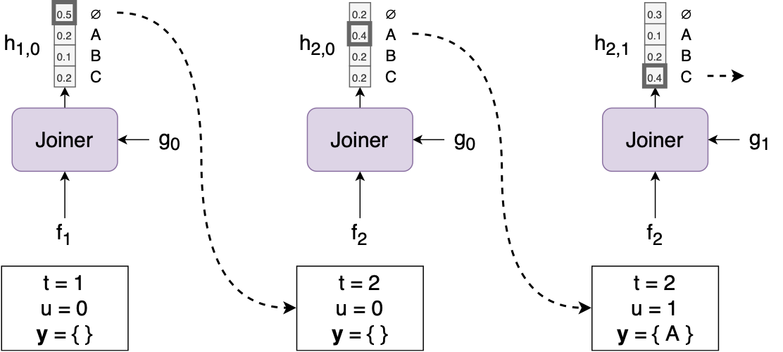
The RNN-T model comprises three modules: an encoder, a decoder, and a joiner network. Notably, the predictor in RNN-T operates in an autoregressive manner- meaning the previous output generated by the joiner is fed back into the predictor in order to predict the next output.
The joiner network combines the outputs of the encoder and predictor, generating a probability distribution over all labels and a null output (\(\phi\)). Note that the predictor relies only on \(\mathbf{y}\) (labels from the text transcript) rather than both \(\mathbf{x}\) and \(\mathbf{y}\), unlike attention-based models. This means one can pre-train the predictor model on a large amount of text.
Greedy Search Algorithm
During the inference phase, RNN-T employs a greedy search algorithm. At each time step \(t\), decisions are made by maximizing computed probabilities. If a label is selected, it is appended to the output sequence \(y\); otherwise, if a blank label \(\phi\) is encountered we move to the next time-step, maintaining the sequential prediction process.
Starting with \(t=1\), \(u=0\), and an empty set \(y={}\), the initial output (\(h_{t,u}\) computed using \(f_t\) and \(g_t\)) unfolds with two scenarios:
- If \(\arg \max(h_{t,u})\) corresponds to a label (let’s say \([A]\)), then \(y={A}\), and the time step \(t\) remains at 1.
- If \(\arg \max(h_{t,u})\) is \(\phi\) (indicating a blank label), the predictor advances to the next time step, making \(t=2\), i.e., \(t\) increments by 1.

Training Dynamics
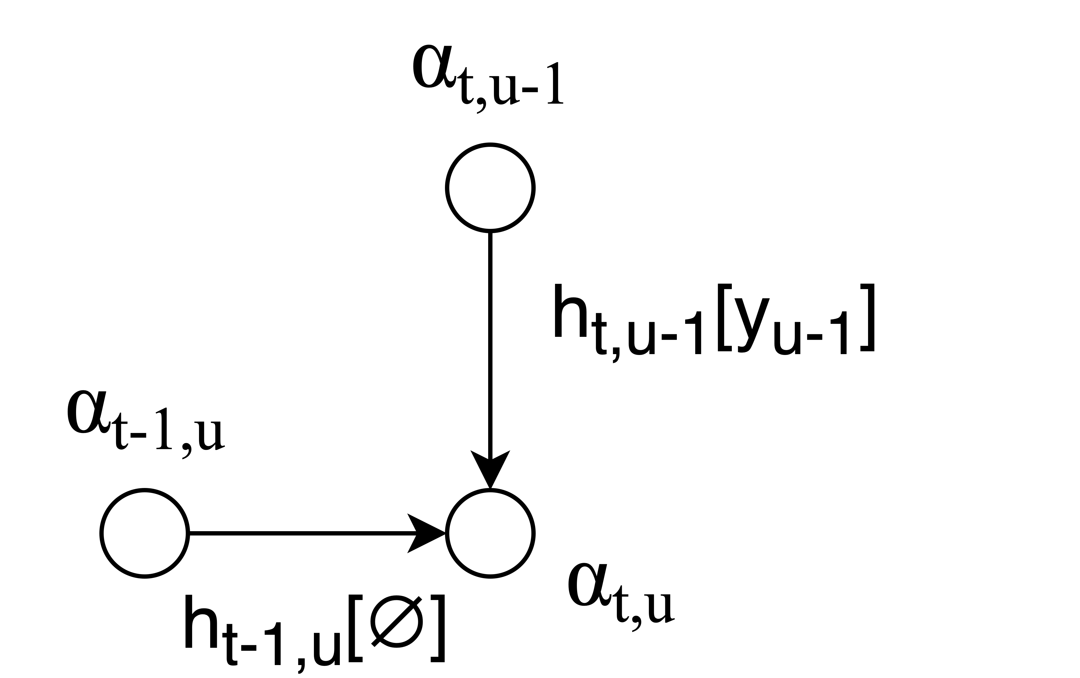
Training RNN-T involves horizontal transitions for blank labels and vertical transitions for actual labels. The forward variable \(\alpha_{t,u}\) is computed using a recursive formula:
\[\alpha_{t,u} = h_{t, u-1} [y_{u-1}] \cdot \alpha_{t, u-1} + h_{t-1, u}[\phi] \cdot\alpha_{t-1, u}\]The above equation represents the computation of the forward variable \(\alpha_{t,u}\). Following this computation, we derive the probability \(p(\mathbf{y}|\mathbf{x})\), indicating the likelihood of a label given acoustic features, expressed as
\[p(\mathbf{y}|\mathbf{x}) = \alpha_{T,U} \cdot h_{T,U} [\phi]\]
State-of-the-Art: Pruned RNN-T
A noteworthy advancement is introduced in the paper titled ‘‘Pruned RNN-T for fast, memory-efficient ASR training’’ (link). This involves a stateless prediction network, an alternative to the traditional RNN decoder. The predictor, similar to a bi-gram language model, simplifies the architecture by relying solely on the last output symbol, eliminating the need for recurrent layers. Its sole purpose lies in assisting the model to output an actual label or a blank label.
Alignment in RNN-T
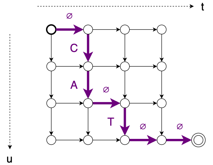
The Transducer in RNN-T defines a set of possible monotonic alignments between the input sequence \(x\) and the output sequence \(y\). These alignments, illustrated using an example with the word “CAT,” showcase the model’s ability to align labels with input features.

(This example along with the equation has been taken from Lugosch, 2020)
We can calculate the probability of one of these alignments by multiplying together the values of each edge along the path:
\[\mathbf{z} = \phi, C, A, \phi, T, \phi, \phi\] \[p(\mathbf{z} | \mathbf{x}) = h_{1,0}[\phi] \cdot h_{2,0}[C] \cdot h_{2,1}[A] \cdot h_{2,2}[\phi] \cdot h_{3,2}[T] \cdot h_{3,3}[\phi] \cdot h_{4,3}[\phi]\]Conclusion
As we conclude the post, you now possess at least a basic understanding of RNN-T models and the functional principle behind it in the context of Automatic Speech Recognition (ASR). The way encoder, decoder, and joiner networks work together, along with features like stateless predictions, makes RNN-T easier to train.